Die Ebene \(F\) schneidet die \(x_{1}x_{2}\)-Ebene in der Geraden \(g\). Bestimmen Sie eine Gleichung von \(g\).
(zur Kontrolle: \(g \colon \overrightarrow{X} = \begin{pmatrix} 30 \\ 0 \\ 0 \end{pmatrix} + \lambda \cdot \begin{pmatrix} 1 \\ -3 \\ 0 \end{pmatrix}, \; \lambda \in \mathbb R\))
(3 BE)
Lösung zu Teilaufgabe e
\(F \colon 3x_{1} + x_{2} + 5x_{3} - 90 = 0\) (vgl. Teilaufgabe d)
Die Gleichung der Ebene \(F\) liegt in der Normalenform in Koordinatendarstellung vor. Für die Bestimmung der Schnittgerade der Ebene \(F\) und der \(x_{1}x_{2}\)-Ebene, kann die Gleichung der \(x_{1}x_{2}\)-Ebene entweder ebenfalls in der Normalenform in Koordinatendarstellung oder in der Parameterform formuliert werden.
1. Möglichkeit: Gleichung der \(x_{1}x_{2}\)-Ebene in Normalenform in Koordinatendarstellung
\[F \colon 3x_{1} + x_{2} + 5x_{3} - 90 = 0\]
\[x_{1}x_{2}\text{-Ebene}\,\colon x_{3} = 0\]
Die Schnittgerade ist die Menge aller gemeinsamer Punkte beider Ebenen. Die Ebenengleichungen bilden diesbezüglich ein lineares Gleichungssystem.
\[\Rightarrow \enspace \left\{ \begin{align*} \text{I} & & & \quad \;3x_{1} + x_{2} + 5x_{3} - 90 = 0 \\[0.8em] \textcolor{#e9b509}{\text{II}} & & \wedge \enspace & \qquad \qquad \qquad \enspace \, \textcolor{#e9b509}{x_{3} \qquad \; = 0} \end{align*} \right.\]
In diesem Fall ergibt sich durch Einsetzen von Gleichung II in Gleichung I eine unterbestimmte Gleichung für die zu bestimmenden Koordinaten \(x_{1}\) und \(x_{2}\).
\[\begin{align*}\textcolor{#e9b509}{\text{II}}\text{ in I}\,\colon\; 3x_{1} + x_{2} + 5 \cdot \textcolor{#e9b509}{0} - 90 &= 0 \\[0.8em] 3x_{1} + x_{2} - 90 &= 0 \end{align*}\]
Die unterbestimmte Gleichung lässt sich nur lösen, indem eine der beiden Koordinaten \(x_{1}\) oder \(x_{2}\) als variabel festgelegt wird, beispielsweise mit \(x_{1} = \lambda\) oder \(x_{2} = \lambda\), jeweils \(\lambda \in \mathbb R\).
Mit \(\textcolor{#89ba17}{x_{1} = \lambda}; \; \lambda \in \mathbb R\) folgt:
\[3 \cdot \textcolor{#89ba17}{\lambda} + x_{2} - 90 = 0 \enspace \Leftrightarrow \enspace \textcolor{#cc071e}{x_{2} = 90 - 3\lambda}\]
Ortsvektor eines beliebigen gemeinsamen Punktes \(X\) der Ebene \(F\) und der \(x_{1}x_{2}\)-Ebene formulieren:
\[\begin{align*}\overrightarrow{X} &= \begin{pmatrix} \textcolor{#89ba17}{x_{1}} \\ \textcolor{#cc071e}{x_{2}} \\ \textcolor{#e9b509}{x_{3}} \end{pmatrix} = \begin{pmatrix} \textcolor{#89ba17}{\lambda} \\ \textcolor{#cc071e}{90 - 3\lambda} \\ \textcolor{#e9b509}{0} \end{pmatrix} = \begin{pmatrix} \enspace0 + 1 \cdot \lambda \\ 90 - 3 \cdot \lambda \\ \enspace0 + 0 \cdot \lambda \end{pmatrix} \\[0.8em] &= \begin{pmatrix} 0 \\ 90 \\ 0 \end{pmatrix} + \lambda \cdot \begin{pmatrix} 1 \\ -3 \\ 0 \end{pmatrix} \end{align*}\]
Damit lautet einen Gleichung der Schnittgeraden \(g\) der Ebene \(F\) und der \(x_{1}x_{2}\)-Ebene:
\[g \colon \overrightarrow{X} = \begin{pmatrix} 0 \\ 90 \\ 0 \end{pmatrix} + \lambda \cdot \begin{pmatrix} 1 \\ -3 \\ 0 \end{pmatrix}; \; \lambda \in \mathbb R\]
Oder mit \(\textcolor{#89ba17}{x_{2} = \lambda}; \; \lambda \in \mathbb R\) folgt:
\[3x_{1} + \textcolor{#89ba17}{\lambda} - 90 = 0 \enspace \Leftrightarrow \enspace \textcolor{#cc071e}{x_{1} = 30 - \frac{1}{3}\lambda}\]
Ortsvektor eines beliebigen gemeinsamen Punktes \(X\) der Ebene \(F\) und der \(x_{1}x_{2}\)-Ebene formulieren:
\[\begin{align*}\overrightarrow{X} &= \begin{pmatrix} \textcolor{#cc071e}{x_{1}} \\ \textcolor{#89ba17}{x_{2}} \\ \textcolor{#e9b509}{x_{3}} \end{pmatrix} = \begin{pmatrix} \textcolor{#cc071e}{30 - \frac{1}{3}\lambda} \\ \textcolor{#89ba17}{\lambda} \\ \textcolor{#e9b509}{0} \end{pmatrix} = \begin{pmatrix} 30 - \frac{1}{3} \cdot \lambda \\ \enspace0 + 1 \cdot \lambda \\ \enspace0 + 0 \cdot \lambda \end{pmatrix} \\[0.8em] &= \begin{pmatrix} 30 \\ 0 \\ 0 \end{pmatrix} + \lambda \cdot \begin{pmatrix} -\frac{1}{3} \\ 1 \\ 0 \end{pmatrix} \\[0.8em] &= \begin{pmatrix} 30 \\ 0 \\ 0 \end{pmatrix} + \underbrace{\lambda \cdot \left(-\frac{1}{3}\right)}_{\lambda} \cdot \begin{pmatrix} 1 \\ -3 \\ 0 \end{pmatrix} \quad \text{(Schritt optional)} \\[0.8em] &= \begin{pmatrix} 30 \\ 0 \\ 0 \end{pmatrix} + \lambda \cdot \begin{pmatrix} 1 \\ -3 \\ 0 \end{pmatrix} \end{align*}\]
Damit lautet einen weitere Gleichung der Schnittgeraden \(g\) der Ebene \(F\) und der \(x_{1}x_{2}\)-Ebene:
\[g \colon \overrightarrow{X} = \begin{pmatrix} 30 \\ 0 \\ 0 \end{pmatrix} + \lambda \cdot \begin{pmatrix} 1 \\ -3 \\ 0 \end{pmatrix}; \; \lambda \in \mathbb R\]
(vgl. Kontrollergebnis)
2. Möglichkeit: Gleichung der \(x_{1}x_{2}\)-Ebene in Parameterform
Beispielsweise erhält man mit dem Aufpunkt \(O(0|0|0)\) sowie den beiden linear unabhängigen Richtungsvektoren \(\overrightarrow{u} = \begin{pmatrix} 1 \\ 0 \\ 0 \end{pmatrix}\) und \(\overrightarrow{v} = \begin{pmatrix} 0 \\ 1 \\ 0 \end{pmatrix}\) eine Gleichung der \(x_{1}x_{|2}\)-Ebene in Parameterform.
Ebenengleichung in Parameterform (vgl. Merkhilfe)
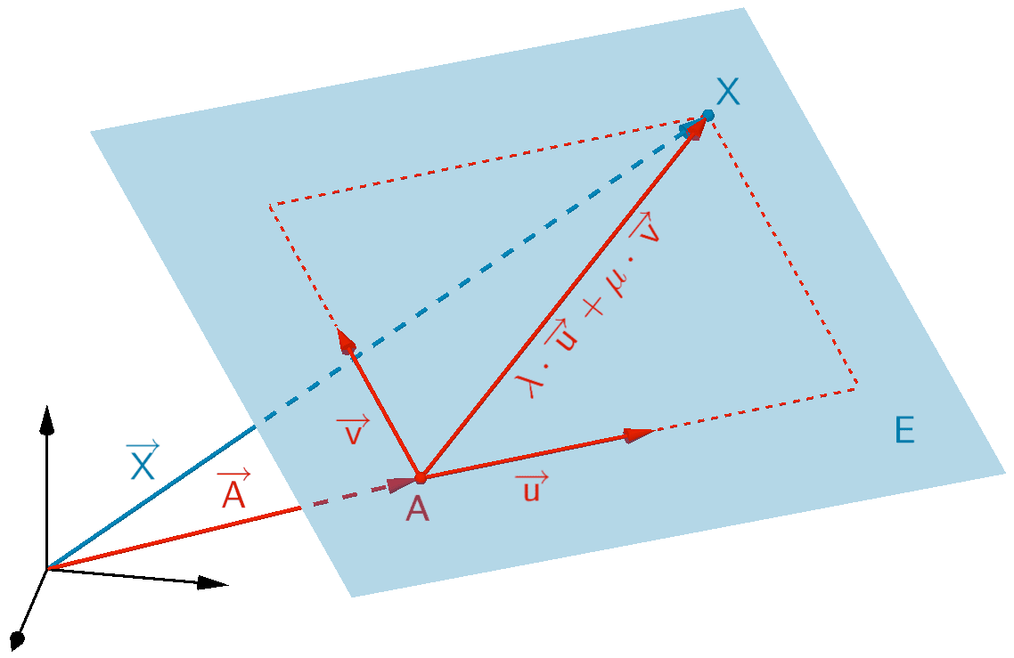
Jede Ebene \(E\) kann durch eine Gleichung in der sogenannten Parameterform
\(E \colon \overrightarrow{X} = \overrightarrow{A} + \lambda \cdot \overrightarrow{u} + \mu \cdot \overrightarrow{v} \enspace\) mit den Parametern \(\lambda, \mu \in \mathbb R\) beschrieben werden.
Dabei ist \(\overrightarrow{A}\) der Ortsvektor eines Aufpunkts (Stützvektor) der Ebene. \(\overrightarrow{u}\) und \(\overrightarrow{v}\) sind zwei linear unabhängige Richtungsvektoren (Spannvektoren).
\[\begin{align*}x_{1}x_{2}\text{-Ebene}\colon \overrightarrow{X} &= \overrightarrow{O} + \mu \cdot \overrightarrow{u} + \tau \cdot \overrightarrow{v}; \; \mu, \tau \in \mathbb R \\[0.8em] x_{1}x_{2}\text{-Ebene}\colon \overrightarrow{X} &= \begin{pmatrix} 0 \\ 0 \\ 0 \end{pmatrix} + \mu \cdot \begin{pmatrix} 1 \\ 0 \\ 0 \end{pmatrix} + \tau \cdot \begin{pmatrix} 0 \\ 1 \\ 0 \end{pmatrix}; \; \mu, \tau \in \mathbb R \end{align*}\]
Durch Einsetzen der Koordinaten des Ortsvektors \(\overrightarrow{X}\) der Gleichung der \(x_{1}x_{2}\)-Ebene in Parameterform in die Gleichung der Ebene \(F\) in Normalenform in Koordinatendarstellung ergibt sich eine Gleichung, welche die Parameter \(\mu\) und \(\tau\) enthält.
\[F \colon 3x_{1} + x_{2} + 5x_{3} - 90 = 0\]
\[\begin{align*}x_{1}x_{2}\text{-Ebene}\colon \overrightarrow{X} &= \begin{pmatrix} 0 \\ 0 \\ 0 \end{pmatrix} + \mu \cdot \begin{pmatrix} 1 \\ 0 \\ 0 \end{pmatrix} + \tau \cdot \begin{pmatrix} 0 \\ 1 \\ 0 \end{pmatrix}; \; \mu, \tau \in \mathbb R \\[0.8em] &= \begin{pmatrix} \textcolor{#cc071e}{\mu} \\ \textcolor{#e9b509}{\tau} \\ \textcolor{#89ba17}{0} \end{pmatrix} \end{align*}\]
\[\begin{align*} F \cap x_{1}x_{2}\text{-Ebene}\colon 3 \cdot \textcolor{#cc071e}{\mu} + \textcolor{#e9b509}{\tau} + 5 \cdot \textcolor{#89ba17}{0} - 90 &= 0 \\[0.8em] 3\mu + \tau - 90 &= 0 \end{align*}\]
Die Gleichung wird entweder nach dem Parameter \(\mu\) oder nach dem Parameter \(\tau\) aufgelöst und das Ergebnis in die Gleichung der \(x_{1}x_{2}\)-Ebene in Parameterform eingesetzt (Ersetzen eines Parameters). Anschließen lässt sich daraus die Gleichung der Schnittgeraden \(g\) in Parameterform formulieren.
Gleichung nach dem Parameter \(\mu\) auflösen:
\[3\mu + \tau - 90 = 0 \enspace \Leftrightarrow \enspace \textcolor{#0087c1}{\mu = 30 - \frac{1}{3}\tau}\]
\(\textcolor{#0087c1}{\mu = 30 - \dfrac{1}{3}\tau}\) in die Gleichung der \(x_{1}x_{2}\)-Ebene einsetzen:
\[x_{1}x_{2}\text{-Ebene}\colon \overrightarrow{X} = \begin{pmatrix} 0 \\ 0 \\ 0 \end{pmatrix} + \textcolor{#0087c1}{\mu} \cdot \begin{pmatrix} 1 \\ 0 \\ 0 \end{pmatrix} + \tau \cdot \begin{pmatrix} 0 \\ 1 \\ 0 \end{pmatrix}; \; \mu, \tau \in \mathbb R\]
\[\begin{align*}g \colon \overrightarrow{X} &= \begin{pmatrix} 0 \\ 0 \\ 0 \end{pmatrix} + \textcolor{#0087c1}{(30 - \frac{1}{3}\tau)} \cdot \begin{pmatrix} 1 \\ 0 \\ 0 \end{pmatrix} + \tau \cdot \begin{pmatrix} 0 \\ 1 \\ 0 \end{pmatrix} \\[0.8em] g \colon \overrightarrow{X} &= \begin{pmatrix} 0 \\ 0 \\ 0 \end{pmatrix} + \begin{pmatrix} \textcolor{#0087c1}{30} \\ \textcolor{#0087c1}{0} \\ \textcolor{#0087c1}{0} \end{pmatrix} + \textcolor{#0087c1}{\tau} \cdot \begin{pmatrix} \textcolor{#0087c1}{-\frac{1}{3}} \\ \textcolor{#0087c1}{0} \\ \textcolor{#0087c1}{0} \end{pmatrix} + \tau \cdot \begin{pmatrix} 0 \\ 1 \\ 0 \end{pmatrix} \\[0.8em] g \colon \overrightarrow{X} &= \begin{pmatrix} 30 \\ 0 \\ 0 \end{pmatrix} + \tau \cdot \begin{pmatrix} -\frac{1}{3} \\ 1 \\ 0 \end{pmatrix} \\[0.8em] g \colon \overrightarrow{X} &= \begin{pmatrix} 30 \\ 0 \\ 0 \end{pmatrix} + \underbrace{\tau \cdot \left( -\frac{1}{3} \right)}_{\tau} \cdot \begin{pmatrix} 1 \\ -3 \\ 0 \end{pmatrix} \quad \text{(Schritt optional)} \\[0.8em] g \colon \overrightarrow{X} &= \begin{pmatrix} 30 \\ 0 \\ 0 \end{pmatrix} + \tau \cdot \begin{pmatrix} 1 \\ -3 \\ 0 \end{pmatrix} \end{align*}\]
(vgl. Kontrollergebnis)
Oder Gleichung nach dem Parameter \(\tau\) auflösen:
\[3\mu + \tau - 90 = 0 \enspace \Leftrightarrow \enspace \textcolor{#0087c1}{\tau = 90 - 3\mu}\]
\(\textcolor{#0087c1}{\tau = 90 - 3\mu}\) in die Gleichung der \(x_{1}x_{2}\)-Ebene einsetzen:
\[x_{1}x_{2}\text{-Ebene}\colon \overrightarrow{X} = \begin{pmatrix} 0 \\ 0 \\ 0 \end{pmatrix} + \mu \cdot \begin{pmatrix} 1 \\ 0 \\ 0 \end{pmatrix} + \textcolor{#0087c1}{\tau} \cdot \begin{pmatrix} 0 \\ 1 \\ 0 \end{pmatrix}; \; \mu, \tau \in \mathbb R\]
\[\begin{align*} g \colon \overrightarrow{X} &= \begin{pmatrix} 0 \\ 0 \\ 0 \end{pmatrix} + \mu \cdot \begin{pmatrix} 1 \\ 0 \\ 0 \end{pmatrix} + \textcolor{#0087c1}{(90 - 3\mu)} \cdot \begin{pmatrix} 0 \\ 1 \\ 0 \end{pmatrix} \\[0.8em] g \colon \overrightarrow{X} &= \begin{pmatrix} 0 \\ 0 \\ 0 \end{pmatrix} + \mu \cdot \begin{pmatrix} 1 \\ 0 \\ 0 \end{pmatrix} + \begin{pmatrix} \textcolor{#0087c1}{0} \\ \textcolor{#0087c1}{90} \\ \textcolor{#0087c1}{0} \end{pmatrix} + \textcolor{#0087c1}{\mu} \cdot \begin{pmatrix} \textcolor{#0087c1}{0} \\ \textcolor{#0087c1}{-3} \\ \textcolor{#0087c1}{0} \end{pmatrix} \\[0.8em] g \colon \overrightarrow{X} &= \begin{pmatrix} 0 \\ 90 \\ 0 \end{pmatrix} + \mu \cdot \begin{pmatrix} 1 \\ -3 \\ 0 \end{pmatrix}; \; \mu \in \mathbb R \end{align*}\]

